Working solutions, not slides.
Process redesign, process mining and Power BI reporting first, then what comes next once reporting is reliable: capacity, agent monitoring and delivery. All examples use sample data.
See a redesigned process outrun the current one.
The same requests arrive at two versions of a request process. The current one finds missing information late and has a decision queue nobody owns. The redesigned one checks information at intake and gives the queue an owner. Push demand up and watch which process breaks first.
Browser simulation · illustrative parameters, not client data
Request journey: current vs redesigned
Each dot is a request moving between steps; red arcs are requests sent back for missing information.
How we use this: we calibrate the same kind of model with your measured volumes and step times (from system timestamps or a time study), then test the redesign before anyone changes how they work.
See how the process really runs.
Process mining rebuilds the real process from system event logs: every case, every activity and when it happened. This report follows the layout of the Power Automate Process Mining report in Power BI: summary measures, the process map with frequency, performance and rework layers, time analysis and variant DNA.
Browser recreation with a synthetic event log of 1,200 invoices · not Microsoft's visual, not client data
Invoice processing
Click any activity, path or variant to cross-filter the report; Ctrl+click adds variants. In a client project this runs on the Microsoft Process Map visual over your own event log, with the findings feeding the process redesign.
Twenty live dashboards, one decision on each.
Working reports, not screenshots: governed measures, clear pages and a named decision on each, across process, finance, operations, quality and platform work. Filter by area, then explore one here or full screen.
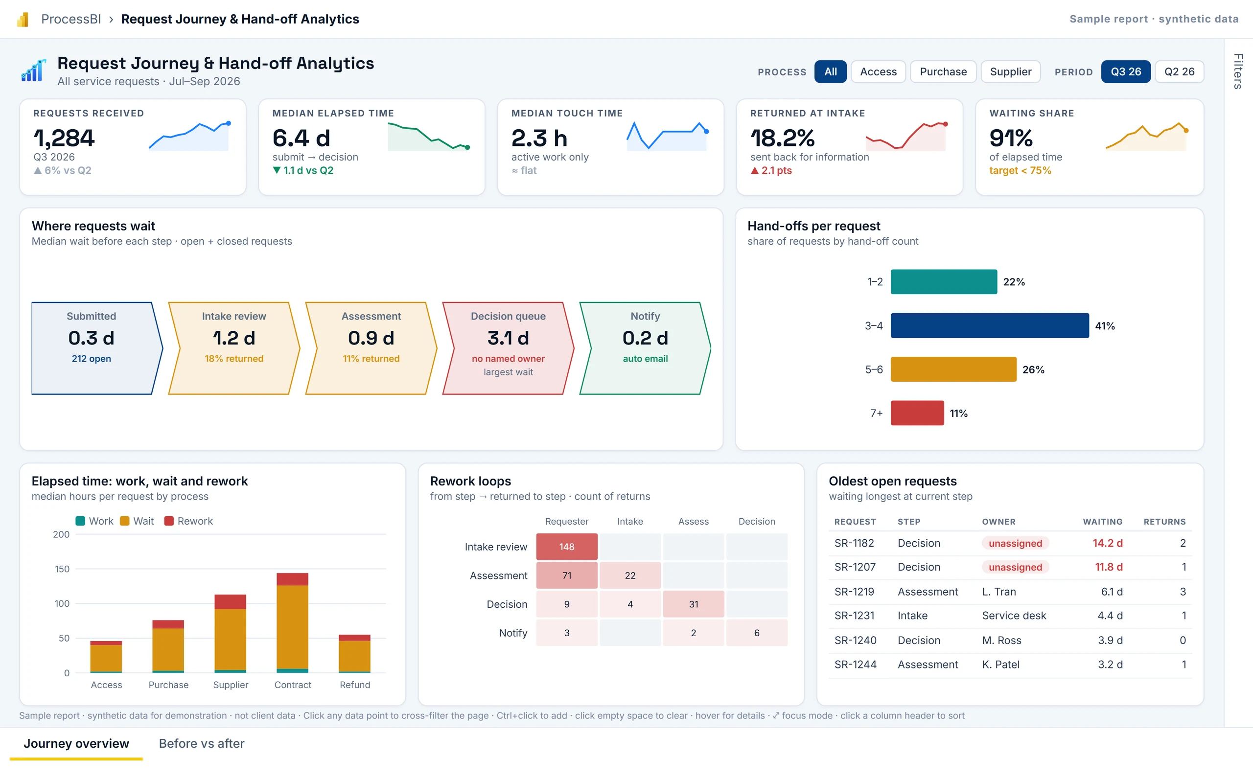
Synthetic sample data. Click any bar, point or row to cross-filter; hover for details.
Capacity that follows the workload.
Use the capacity you already have before paying for more. The policy combines usage signals and scheduled workload windows to decide when to scale up, hold capacity and safely scale down.
A day of changing demand
Capacity policy
- 01 · Prepare for ETLIncrease ahead of the planned overnight workload. Hold while background consumption settles.
- 02 · Use the headroomSupport morning reports, then use available capacity before requesting another increase.
- 03 · Respond to pressureRaise the allocation when sustained demand warrants it, within agreed limits.
- 04 · Scale down safelyCheck workload completion, smoothed consumption and cooldown before reducing capacity.
A low point on a usage graph is not enough to justify scaling down. The policy must consider smoothing, carryforward usage, workload health and reporting/licensing requirements. The timings shown here are an example, not recommended thresholds. This is capacity resizing, not Microsoft's separate Spark autoscale billing feature.
View the example capacity schedule
| Time | Allocation | Policy intent |
|---|---|---|
| 00:00 | F8 | Quiet period |
| 01:00 | F64 | Prepare for scheduled ETL |
| 06:00 | F16 | Reduce after workload checks |
| 08:00 | F32 | Morning reporting window |
| 12:00 | F16 | Lower sustained demand |
| 15:30 | F64 | Respond to rising pressure |
| 19:00 | F32 | Hold while work settles |
| 21:00 | F8 | Reduce after cooldown and checks |
The cost difference in one engagement
These supplied monthly figures are separate from the synthetic usage graph above.
AUD 64,800 annualised difference versus the reserved comparator, if sustained for 12 months.
Read the autoscaling case study →Base: owner-supplied comparison. Reserved: a 40% discount assumption. Autoscaled: client-reported engagement result. These are not guaranteed savings; actual cost depends on workload, region, licensing and billing. A reservation is a billing commitment, not a restriction on resizing.
Monitor AI-agent performance.
Compare response times, error rates and throughput. Select an agent, introduce a sample problem and investigate the signals.
Browser demonstration · synthetic sample data
Watch agents and people move work forward.
See AI agents perform repeatable tasks, pass evidence to people for review and keep the next action visible. Cards move through a scripted sample sprint; open one to inspect the handoff or take control.
Browser demonstration · synthetic sample data
Want this running on your data?
Tell us what you need to see on your own data.
Talk through your project →